
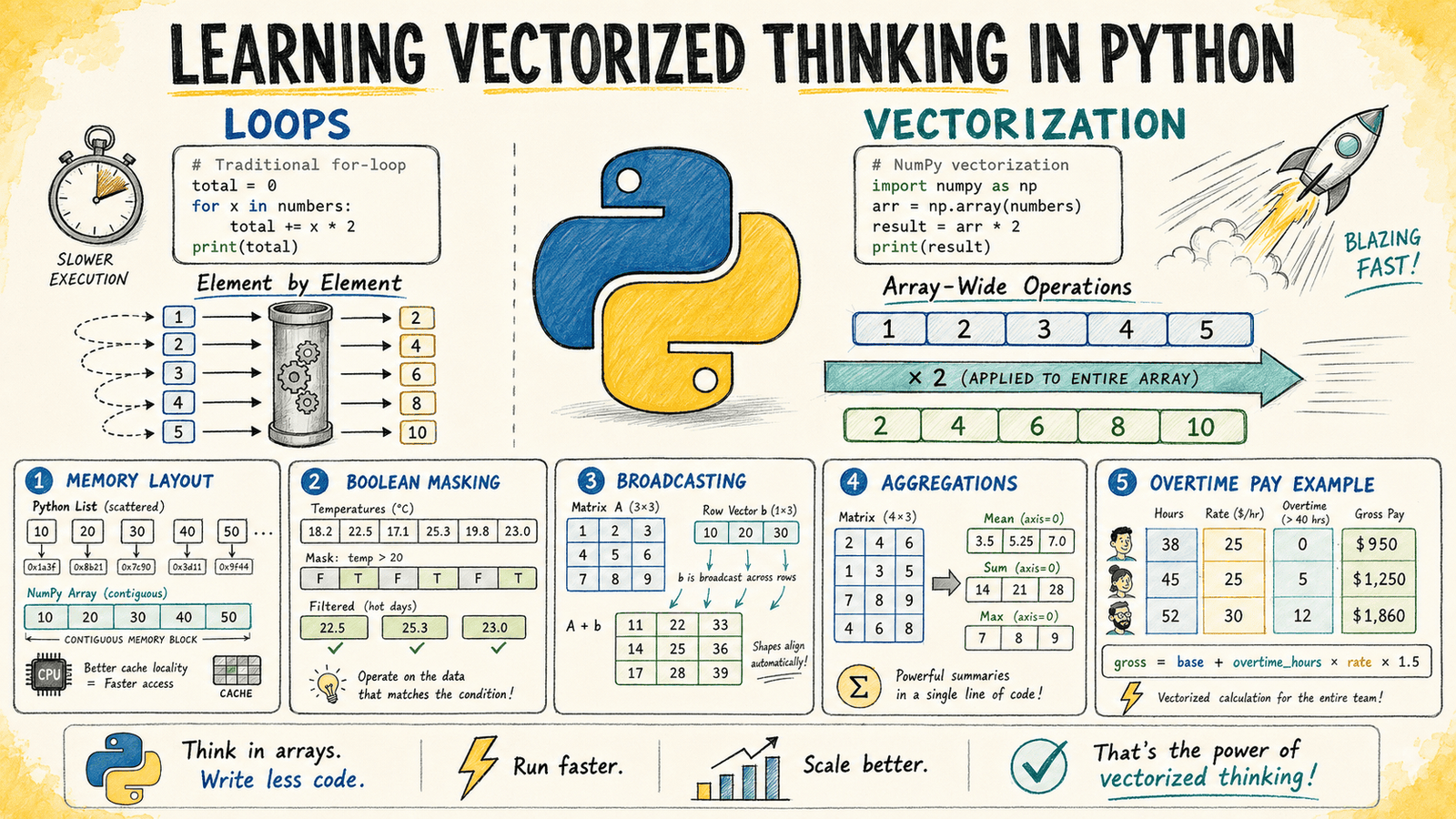
In this article, you will learn how to think in terms of vectorized operations using NumPy, replacing slow Python loops with efficient array-level computations.
Topics we will cover include:
- Why Python loops are slow for numeric data and how NumPy’s C-backed engine addresses this.
- How to apply element-wise operations, boolean masking, and broadcasting to eliminate common loop patterns.
- How to handle multi-condition branching and axis-based aggregation entirely with NumPy functions.
Introduction
You already know how to loop in Python. Loops are simple, readable, and they do exactly what they say. The problem is that at scale, Python loops become too slow. At some point, every developer working with numeric data starts looking for a better approach.
NumPy’s vectorized operations provide that alternative. Instead of telling Python what to do element by element, you describe the transformation at the array level and let NumPy’s C-backed engine apply it across all elements efficiently.
This article teaches vectorized thinking through a set of examples. You’ll see the loop-based version, its vectorized equivalent, and the reasoning behind translating one into the other.
You can find the complete code for these examples on GitHub.
Understanding Why Loops Are Slow In Python
It helps to start by understanding why the loop you are replacing is slow.
Python is dynamically typed. Every time you write an operation like x * 2 inside a loop, Python must determine the type of x, find the correct multiplication method, execute it, and create a new Python object for the result.
That overhead is insignificant when working with a small number of elements. But when the same operation runs across millions of values, those repeated Python-level operations add up quickly.
NumPy arrays work differently. They store elements as raw numbers in a contiguous block of memory, similar to how arrays are stored in C. When you write arr * 2, NumPy passes the entire array to a compiled C routine that applies the operation without Python overhead for each individual item.
The computation runs closer to compiled code speed rather than interpreted Python speed.
Applying Operations Element By Element
A common first step with numeric data is applying the same formula to every value in a list.
Consider a simple example: you have a list of product prices and need to apply a 12% tax rate to each item.
Loop Version
The traditional approach iterates through each price, calculates the taxed value, and appends the result to a new list.
|
prices = [12.99, 45.00, 7.49, 129.99, 3.25, 89.50]
taxed = [] for price in prices: taxed.append(round(price * 1.12, 2))
print(taxed) |
Output:
|
[14.55, 50.4, 8.39, 145.59, 3.64, 100.24] |
Vectorized Version
The vectorized approach replaces the loop with a single operation on a NumPy array. When you write prices * 1.12, NumPy applies the multiplication to every element automatically.
|
import numpy as np
prices = np.array([12.99, 45.00, 7.49, 129.99, 3.25, 89.50]) taxed = np.round(prices * 1.12, 2)
print(taxed) |
Output:
|
[ 14.55 50.4 8.39 145.59 3.64 100.24] |
The output is identical, but the approach scales much better. For large arrays containing millions of prices, the vectorized version can be dramatically faster than the loop-based equivalent.
The important mental shift is moving from:
“For each price, perform this calculation.”
to:
“Apply this transformation to the entire array of prices.”
The array becomes the unit of computation rather than the individual element.
Using Boolean Masking For Conditional Logic
Loops often contain if statements that check each value individually. The vectorized equivalent is a boolean mask: an array of True and False values generated from a comparison.
A boolean mask can then be used to filter values or update selected elements without writing a loop.
Consider a weather monitoring system that records hourly temperatures. You want to flag every reading above 38°C as a heat alert.
Loop Version
The loop approach checks each temperature value and builds a separate list of alert flags.
|
readings = [34.1, 38.5, 37.2, 39.0, 36.8, 40.1, 35.5]
alerts = [] for temp in readings: alerts.append(temp > 38.0)
print(alerts) |
Output:
|
[False, True, False, True, False, True, False] |
Vectorized Version
With NumPy, comparing an array directly creates the boolean mask automatically. There is no explicit loop and no repeated append() operation.
|
import numpy as np
readings = np.array([34.1, 38.5, 37.2, 39.0, 36.8, 40.1, 35.5])
alerts = readings > 38.0
print(alerts) print(“Alert readings:”, readings[alerts]) |
Output:
|
[False True False True False True False] Alert readings: [38.5 39. 40.1] |
The mask can immediately index back into the original array and return only the values that matched the condition.
This pattern is one of the most important ideas in vectorized programming:
Compute a mask, then use that mask to select or modify values.
It replaces many of the conditional checks you would normally write inside a loop.
For conditional assignment, np.where() provides a compact alternative. For example, the following operation sets high temperatures to 38.0 while leaving other values unchanged:
|
np.where(readings > 38.0, 38.0, readings) |
Broadcasting Across Different Array Shapes
Broadcasting is NumPy’s mechanism for applying operations between arrays with different shapes without creating unnecessary copies.
It can feel more abstract at first, but it removes many nested loops that would otherwise be needed to align data structures manually.
Consider a practical example. Imagine you have click-through rate data for five marketing campaigns across three channels: email, social, and search. You want to normalize each channel by dividing values by the maximum value in that column.
Loop Version
The loop-based approach processes each column separately.
|
1 2 3 4 5 6 7 8 9 10 11 12 13 14 15 16 17 18 19 |
import numpy as np
# rows = campaigns, columns = channels (email, social, search) ctr = np.array([ [0.042, 0.031, 0.078], [0.019, 0.055, 0.091], [0.033, 0.047, 0.063], [0.061, 0.028, 0.085], [0.025, 0.039, 0.070], ])
# Loop version: normalize each column separately normalized_loop = np.zeros_like(ctr)
for col in range(ctr.shape[1]): col_max = ctr[:, col].max() normalized_loop[:, col] = ctr[:, col] / col_max
print(normalized_loop) |
Output:
|
[[0.68852459 0.56363636 0.85714286] [0.31147541 1. 1. ] [0.54098361 0.85454545 0.69230769] [1. 0.50909091 0.93406593] [0.40983607 0.70909091 0.76923077]] |
The result is correct, but the logic requires iterating over the columns.
Vectorized Version
The broadcasting approach calculates the column maximums as a one-dimensional array and divides the entire matrix in a single operation.
|
col_maxima = ctr.max(axis=0)
normalized = ctr / col_maxima
print(normalized) |
Output:
|
[[0.68852459 0.56363636 0.85714286] [0.31147541 1. 1. ] [0.54098361 0.85454545 0.69230769] [1. 0.50909091 0.93406593] [0.40983607 0.70909091 0.76923077]] |
NumPy sees a (5, 3) array divided by a (3,) array and automatically aligns the shapes. The one-dimensional array is treated conceptually as a row vector and applied across all five rows.
No actual copy is created. NumPy handles the operation efficiently inside its compiled layer.
The general rule is simple: when a loop exists only to make array shapes line up, broadcasting is often the cleaner solution.
Aggregating Data Along An Axis
Many data tasks involve summarizing rows or columns of a matrix. NumPy’s reduction functions, such as sum(), mean(), max(), and std(), include an axis argument that determines the direction of the reduction.
The axis parameter tells NumPy which dimension to collapse:
axis=0collapses rows, returning one value per column.axis=1collapses columns, returning one value per row.- Leaving
axisunspecified reduces the entire array to a single value.
Continuing with the click-through rate data from the previous example, you can calculate average performance per channel and per campaign without writing any loops.
|
channel_avg = ctr.mean(axis=0) campaign_avg = ctr.mean(axis=1)
print(“Channel averages:”, np.round(channel_avg, 4)) print(“Campaign averages:”, np.round(campaign_avg, 4)) |
Output:
|
Channel averages: [0.036 0.04 0.0774] Campaign averages: [0.0503 0.055 0.0477 0.058 0.0447] |
The output provides both summaries in only two lines. A loop-based approach would require separate iterations for calculating row and column averages.
With NumPy, the axis argument directly expresses the intent of the operation.
Replacing Multi-Condition Loops
Data processing often combines multiple conditions with calculations. Vectorization becomes especially valuable when a loop contains branching logic that handles different cases.
Consider a payroll example. You have employee hours and hourly rates, and you need to calculate gross pay where hours above 40 receive overtime pay at 1.5 times the regular rate.
Loop Version
The loop version checks each employee individually and applies the correct calculation.
|
hours = np.array([38, 45, 40, 52, 33, 41]) rate = np.array([22.50, 18.00, 31.00, 15.50, 27.00, 19.75])
pay_loop = []
for h, r in zip(hours, rate): if h <= 40: pay_loop.append(h * r) else: regular = 40 * r overtime = (h – 40) * r * 1.5 pay_loop.append(regular + overtime)
print([round(p, 2) for p in pay_loop]) |
Output:
|
[np.float64(855.0), np.float64(855.0), np.float64(1240.0), np.float64(899.0), np.float64(891.0), np.float64(819.62)] |
Vectorized Version
The vectorized approach separates the calculation into array operations. Regular pay applies to the first 40 hours, while overtime pay applies only to hours above that threshold.
|
regular_pay = np.minimum(hours, 40) * rate
overtime_pay = np.maximum(hours – 40, 0) * rate * 1.5
gross_pay = np.round(regular_pay + overtime_pay, 2)
print(gross_pay) |
Output:
|
[ 855. 855. 1240. 853.25 891. 839.38] |
The np.minimum() function caps each value at 40, automatically handling employees who did not work overtime.
The np.maximum() function calculates overtime hours by subtracting 40 and replacing negative values with zero, ensuring employees without overtime contribute nothing to the overtime calculation.
The key mental shift is replacing if/else branches with element-wise operations that produce the correct result for every value simultaneously.
Building The Habit Of Vectorized Thinking
Vectorized thinking is a skill that develops with practice. The main challenge is changing your approach from describing how Python should iterate to describing what the array should become.
When you see a loop that processes numeric data, use this checklist:
- Does the operation apply the same formula to every element? Use array arithmetic.
- Does it filter values based on a condition? Use a boolean mask.
- Does it summarize rows or columns? Use
np.sum(),np.mean(), or similar functions with anaxisargument. - Does it operate on arrays with different shapes? Check whether broadcasting can replace the loop.
You should not, however, eliminate every loop in your code. Some problems are naturally iterative, and forcing vectorization can make code harder to understand. Your goal should be to recognize when the array itself can represent the full computation.
From here, the next step is exploring np.vectorize() for functions that do not map naturally to built-in array operations.
You can also learn to vectorize operations in pandas, which builds a column-oriented data structure on top of NumPy arrays and extends the same vectorized model to labeled, mixed-type datasets.